|
|
|
| Title | Use VBA code to make a pie chart in Excel |
|---|
| Description | This example shows how to use VBA code to make a pie chart in Excel. |
|---|
| Keywords | Excel, VBA, pie chart, Microsoft Office |
|---|
| Categories | Office, Graphics |
|---|
|
|
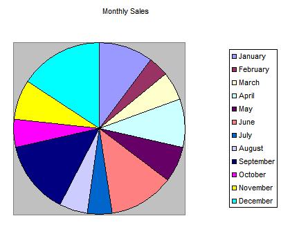
Subroutine MakePieChart builds a pie chart. This example builds a pie chart showing sales per month. It takes as parameters:
- A title to put on the chart.
- A title for the categories to graph (in this example, Month).
- An array of category values (January, February, and so forth).
- The title for the values (in this example, Sales).
- An array of values (the sales per month).
The subroutine first created a new worksheet and names it after the title parameter. It makes column headers in cells A1 and B1, and then copies the categories and values into columns A and B.
The code then builds the chart. It sets the chart's type, data source, and details such as the title.
|
|
Public Sub MakePieChart(ByVal title As String, ByVal _
    category_title As String, category_values() As String, _
    ByVal value_title As String, values() As Single)
Dim work_book As Workbook
Dim last_sheet As Worksheet
Dim new_sheet As Worksheet
Dim r As Integer
Dim min_r As Integer
Dim new_chart As Chart

    ' Make a new worksheet.
    Set work_book = Application.ActiveWorkbook
    Set last_sheet = _
        work_book.Sheets(work_book.Sheets.Count)
    Set new_sheet = work_book.Sheets.Add(after:=last_sheet)
    new_sheet.Name = title

    ' Make the column headers.
    new_sheet.Cells(1, 1) = category_title
    new_sheet.Cells(1, 2) = value_title

    With new_sheet.Range("A1:B1")
        .HorizontalAlignment = xlCenter ' Centered.
        With .Font
            .FontStyle = "Bold"         ' Bold.
            .Size = .Size + 2           ' Bigger.
            .ColorIndex = 3             ' Red.
        End With
    End With

    ' Write the data.
    min_r = 2 - LBound(category_values)
    For r = LBound(category_values) To _
        UBound(category_values)
        new_sheet.Cells(r + min_r, 1) = category_values(r)
    Next r

    min_r = 2 - LBound(values)
    For r = LBound(values) To UBound(values)
        new_sheet.Cells(r + min_r, 2) = values(r)
    Next r

    ' Make the chart.
    Set new_chart = Charts.Add()
    ActiveChart.ChartType = xlPie
    ActiveChart.SetSourceData _
        Source:=new_sheet.Range("A1:B" & UBound(values) + _
            min_r), _
        PlotBy:=xlColumns
    ActiveChart.Location Where:=xlLocationAsObject, _
        Name:=title
    With ActiveChart
        .HasTitle = True
        .ChartTitle.Characters.Text = title
    End With

    ' Move the chart.
    new_sheet.Shapes(1).IncrementLeft -80
    new_sheet.Shapes(1).IncrementTop -140
End Sub
|
| |

|
| |
|
|