The following examples show how to fit a set of points that lie along a line or polynomial equation:
The basic idea behind these algorithms is to:
- Calculate an error function containing unknown coefficients
- Find the partial derivatives of the error function with respect to the coefficients
- To find the coefficients that give the smallest error, set the partial derivatives equal to zero and solve for the coefficients
For linear and polynomial least squares, the partial derivatives happen to have a linear form so you can solve them relatively easily by using Gaussian elimination.
But what if the points don't lie along a polynomial? What if the partial derivatives of the error function are not easy to solve? This entry examines such an example.
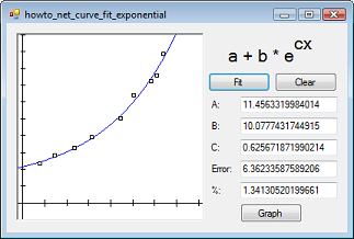
Consider the points in the picture and suppose you want to find values a, b, and c to make the equation F(x) = a + b * ec * x fit the curve. You can begin as before, finding the error function and taking its partial derivatives. The following equation shows the error function.
![Sum[(yi - F(x,a,b,c))^2] = Sum[(yi - (a+b*e^(c*x)))^2]](howto_curve_fit_exponential_eq1.png)
Now you can take the partial derivatives of this function with respect to a, b, and c. For example, the following equation shows the partial derivative with respect to c.
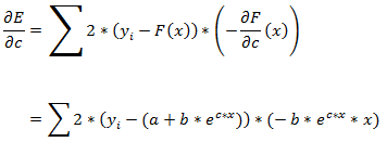
After finding the partial derivatives, you would set them equal to 0 and solve for a, b, and c. Unfortunately the previous equation is a mess. The partial derivatives with respect to a and b are a bit simpler but, frankly, I don't know how to solve the system of these three equations. (If you can solve them, please email me and tell me how.)
The point of setting the partial derivatives of E equal to 0 and solving was to minimize the error function E. Although you can't directly solve the equations, you can use them to minimize E.
This program starts with a guess (a, b, c). It then calculates the partial derivatives at that point to get a gradient vector. The gradient vector <va, vb, vc> gives the error function's direction of maximum increase.
To think of this another way, pretend the error function is a function E(x, y) that defines a surface in three-dimensional space. The gradient <vx, vy> tells the direction to move that increases the function the most. In other words, it tells you how to move directly uphill on the surface.
Conversely the negative of the gradient <-vx, -vy> tells you how to move directly downhill on the surface.
That's what the program does. It calculates the gradient at the guess point (a, b, c) and moves a small distance in the opposite direction. If the value at the new point is greater than the value at the current point, then the program tries moving a smaller distance in the same direction. It continues trying smaller distances until it finds one that works. It then updates (a, b, c) to the new point and starts over.
If you consider the three-dimensional analogy again, the program moves downhill until it can't find any way to more farther downhill or it exceeds a maximum number of moves.
See the code for the details about partial derivatives and how the program controls its search.
There is one piece of the process that's a bit fuzzy. The program picks test points (a, b, c) within an area where I suspect the solution may lie. It then follows the gradients from each of those points and picks the best solution. Where you pick those points depends on the equation F.
The number of points that you pick and the maximum number of iterations that you should use for each point will depend on the shape of the surface defined by the error function E. If the function is relatively smooth, then any initial point should lead eventually to a good solution, so you may only need to pick a few points and follow them for many iterations.
In contrast, if E defines a wrinkly surface with many local minima, then from a given starting point the program may become stuck and not reach a global minimum. In that case, you should pick many initial points and iterate them as long as you can. In the three-dimensional analogy, the difference is between a single smooth hillside and terrain full of bumps, valleys, and sinkholes.
|