Beyond Flatland
By Rod Stephens
[Editor's note: In Rod's past columns, the Algorithmic Adventurer has explained several topics in two-dimensional graphics including least squares curve fitting (June 1997), image rotation (August 1997), and image filtering (November 1997). This month he steps out of flatland into the third dimension.]
Three-dimensional graphics is a complicated subject. Entire books have been dedicated to nothing but three-dimensional graphics. However, the basic techniques used to display simple three-dimensional objects are reasonably straightforward. This article explains those techniques so you can enter the world of three-dimensional graphics.
Homogeneous Coordinates
Homogeneous coordinates allow a program to represent various three-dimensional transformations such as rotation and translation in a homogeneous (uniform) way. The point (x, y, z) in three-dimensional space is represented by the vector [x', y', z', s] where x' = x * s, y' = y * s, and z' = z * s for some scale factor s. For example, the point (2, 7, 5) might be represented by [4, 14, 10, 2] or by [8, 28, 20, 4]. Both of these vectors represent the same point.
Often a point is normalized by dividing the values by the scale factor. The normalized representation of the point (2, 7, 5) is [2, 7, 5, 1].
Three-dimensional transformations such as rotation and translation are represented by matrices. For example, the following matrix represents translation by the distance 3 along the X axis.
| 1 |
0 |
0 |
0 |
| 0 |
1 |
0 |
0 |
| 0 |
0 |
1 |
0 |
| 3 |
0 |
0 |
1 |
To apply a transformation to a point, a program multiplies the transformation matrix by the point's vector. For example, multiplying the previous matrix by the general point [x, y, z, 1] gives [x + 3, y, z, 1]. This shows that applying the matrix to a point translates the point by the distance 3 along the X axis.
Listing 1 shows subroutine PointMatrixMult that multiplies a vector by a matrix. Before returning, the routine normalizes the Rpt array holding the transformed point's homogeneous coordinates.
Sub VectorMatrixMult (Rpt() As Single, _
    Ppt() As Single, A() As Single)
Dim i As Integer
Dim j As Integer
Dim value As Single

    For i = 1 To 4
        value = 0#
        For j = 1 To 4
            value = value + Ppt(j) * A(j, i)
        Next j
        Rpt(i) = value
    Next i

    ' Renormalize the point.
    ' Note that value still holds Rpt(4).
    Rpt(1) = Rpt(1) / value
    Rpt(2) = Rpt(2) / value
    Rpt(3) = Rpt(3) / value
    Rpt(4) = 1#
End Sub
|
Listing 1. Vector-matrix multiplication.
Combining Transformations
One of the most important features of homogeneous coordinates is that you can combine transformations by multiplying their matrices. For example, suppose A, B, C, and D are matrices representing different transformations and P is a vector representing a point. Then (((P * A) * B) * C) * D = P * (A * B * C * D). That means your program can multiply the matrices together first, and then apply the single combined transformation matrix to the point instead of applying the four matrices one at a time.
This may seem like no big deal when you are transforming a single point, but suppose a program needs to display a grid containing 10,000 points. The program could apply each matrix to the points one at a time requiring 40,000 matrix-vector multiplications. If the program first combines the matrices and then multiplies the result by each point, it performs only 10,000 matrix-vector multiplications--about a quarter as many.
Combining transformation matrices like this is very important since the most interesting transformations are made up of many simpler ones. Listing 2 shows the MatrixMatrixMult subroutine that multiplies two transformation matrices.
Sub MatrixMatrixMult (R() As Single, _
    A() As Single, B() As Single)
Dim i As Integer
Dim j As Integer
Dim k As Integer
Dim value As Single

    For i = 1 To 4
        For j = 1 To 4
            value = 0#
            For k = 1 To 4
                value = value + A(i, k) * B(k, j)
            Next k
            R(i, j) = value
        Next j
    Next i
End Sub
|
Listing 2. Matrix-matrix multiplication.
Translation
The general form for a transformation matrix that translates a point distance Tx along the X axis, Ty along the Y axis, and Tz along the Z axis is:
| 1 |
0 |
0 |
0 |
| 0 |
1 |
0 |
0 |
| 0 |
0 |
1 |
0 |
| Tx |
Ty |
Tz |
1 |
You can easily verify this by multiplying the matrix by the point [x, y, z, 1] to get [x + Tx, y + Ty, z + Tz, 1].
Scaling
Scaling (shrinking or stretching) is just as easy as translation. The following matrix represents scaling by the factors of Sx parallel to the X axis, Sy parallel to the Y axis, and Sz parallel to the Z axis.
| Sx |
0 |
0 |
0 |
| 0 |
Sy |
0 |
0 |
| 0 |
0 |
Sz |
0 |
| 0 |
0 |
0 |
1 |
You can verify this by multiplying the matrix by the point [x, y, z, 1] to get [x * Sx, y * Sy, z * Sz, 1].
Rotation
Rotation is a bit more complicated than translation or scaling. To rotate a point you need an axis of rotation and an angle. For example, you might rotate a point through the angle q around the Z axis. During this rotation, the point's Z coordinate does not change. The point's new X and Y coordinates x' and y' are given by:
    x' = x * cos(q) - y * sin(q)
    y' = x * sin(q) + y * cos(q)
You can use these equations to create the following matrix for rotation around the Z axis.
| cos(q) |
sin(q) |
0 |
0 |
| -sin(q) |
cos(q) |
0 |
0 |
| 0 |
0 |
1 |
0 |
| 0 |
0 |
0 |
1 |
When you multiply this matrix by the point [x, y, z, 1] you get [x * cos(q) - y * sin(q), x * sin(q) + y * cos(q), z, 1] as desired.
Similarly you can create matrices for rotation around the X or Y axes. Rotation around the Y axis is represented by:
| cos(q) |
0 |
-sin(q) |
0 |
| 0 |
1 |
0 |
0 |
| sin(q) |
0 |
cos(q) |
0 |
| 0 |
0 |
0 |
1 |
Finally, rotation around the X axis is represented by:
| 1 |
0 |
0 |
0 |
| 0 |
cos(q) |
sin(q) |
0 |
| 0 |
-sin(q) |
cos(q) |
0 |
| 0 |
0 |
0 |
1 |
You can easily verify these matrices if you like.
Parallel Projection
Parallel project onto a coordinate plane is easy. For example, to project a point onto the X-Y plane, a program can simply ignore the point's Z coordinate. The transformation matrix for this projection is:
| 1 |
0 |
0 |
0 |
| 0 |
1 |
0 |
0 |
| 0 |
0 |
0 |
0 |
| 0 |
0 |
0 |
1 |
In practice a program will usually not bother to actually perform the projection. It will simply draw using the point's X and Y coordinates, ignoring the Z coordinates.
Complex Transformations
A program can combine the basic translation, scaling, and rotation matrices to represent more complicated transformations. For example, a transformation that scales an object around a point other than the origin can be created by:
- A translation that moves the point to the origin.
- A scaling.
- The inverse of the translation in step 1.
The program can multiply the matrices representing the three steps together to create a single matrix that represents the scaling.
Similarly a program can use translations and rotations to create a transformation that rotates points around a line other than the coordinate axes.
A program can also combine translations, rotations, and projections to project objects onto a plane other than one of the coordinate planes. For example, suppose you want to project onto a plane that passes through the origin as shown in Figure 1. A vector gives the direction of projection that should be used.
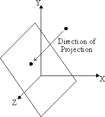
Figure 1. Parallel projection onto a plane.
This projection can be built from the following combination of simpler operations:
- A rotation around the Z axis to make the direction of projection lie parallel to the Y-Z plane.
- A rotation around the X axis to make the direction of projection lie parallel to the Z axis.
- Projection onto the X-Y plane.
Making a Splash
The 3D program shown in Figure 2 draws a parallel projection of the three-dimensional surface z = Cos(Sqr(x2 + y2)). You can find the project's source code in the subscriber download area in ROD298.ZIP [see the Downloads section at the end of this article]. Using the arrow keys, you can make the program display the surface from different directions.
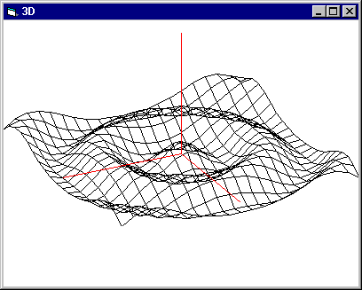
Figure 2. Program 3D displaying a parallel projection of z = Cos(Sqr(x2 + y2)).
The rest of this section explains the program's most important pieces.
The Point3D user-defined type stores information about a three-dimensional point. This structure includes arrays to hold the point's original and transformed homogeneous coordinates.
    Type Point3D
        Coord(1 To 4) As Single ' Original coordinates.
        Trans(1 To 4) As Single ' Translated coordinates.
    End Type
Program 3D stores the surface data in an array of Point3D data structures. It stores three points to represent the coordinate axes in the Axes array.
    Dim Points(Xmin To Xmax, Ymin To Ymax) As Point3D
    Dim Axes(1 To 3) As Point3D
The program displays views of the surface projected onto a plane passing through the origin. It represents the direction of projection with a point of view position having coordinates (EyeX, EyeY, EyeZ). The direction of projection lies along the line from this point to the origin. The resulting projection looks as if your eye is at the point of view looking towards the origin.
Subroutine CalculateTransformation, shown in Listing 3, builds the projection transformation. Using the coordinates of the point of view, it creates two simpler rotation transformations to move the point of view into the Z axis. It multiplies the two rotation matrices to produce the combined transformation.
Sub CalculateTransformation (T() As Single)
ReDim T1(1 To 4, 1 To 4) As Single
ReDim T2(1 To 4, 1 To 4) As Single
Dim r1 As Single
Dim r2 As Single
Dim ctheta As Single
Dim stheta As Single
Dim cphi As Single
Dim sphi As Single

    ' Rotate around the Z axis so the
    ' eye lies in the Y-Z plane.
    r1 = Sqr(EyeX * EyeX + EyeY * EyeY)
    stheta = EyeX / r1
    ctheta = EyeY / r1
    MakeIdentity T1()
    T1(1, 1) = ctheta
    T1(1, 2) = stheta
    T1(2, 1) = -stheta
    T1(2, 2) = ctheta

    ' Rotate around the X axis so the
    ' eye lies in the Z axis.
    r2 = Sqr(EyeX * EyeX + EyeY * EyeY + EyeZ * EyeZ)
    sphi = -r1 / r2
    cphi = -EyeZ / r2
    MakeIdentity T2()
    T2(2, 2) = cphi
    T2(2, 3) = sphi
    T2(3, 2) = -sphi
    T2(3, 3) = cphi

    ' Project along the Z axis. (Actually we do nothing
    ' here. We just ignore the Z coordinate when drawing.)

    ' Combine the transformations.
    MatrixMatrixMult T(), T1(), T2()
End Sub
|
Listing 3. Calculating the projection transformation.
The DrawSurface subroutine, shown in Listing 4, draws the surface. It simply loops through the Points and Axes arrays, connecting the appropriate points. It implicitly performs a projection onto the X-Y plane by ignoring the points' Z coordinates.
Sub DrawSurface ()
ReDim T(1 To 4, 1 To 4) As Single
Dim x As Integer
Dim y As Integer

    ' Calculate the transformation matrix.
    CalculateTransformation T()

    ' Apply the transformation matrix to the points.
    For x = Xmin To Xmax
        For y = Ymin To Ymax
            VectorMatrixMult Points(x, y).Trans(), _
                Points(x, y).Coord(), T()
        Next y
    Next x

    ' Draw lines parallel to the X axis.
    ForeColor = RGB(0, 0, 0)
    For x = Xmin To Xmax
        CurrentX = Points(x, Ymin).Trans(1)
        CurrentY = Points(x, Ymin).Trans(2)
        For y = Ymin + 1 To Ymax
            Line -(Points(x, y).Trans(1), _
                Points(x, y).Trans(2))
        Next y
    Next x

    ' Draw lines parallel to the Y axis.
    For y = Ymin To Ymax
        CurrentX = Points(Xmin, y).Trans(1)
        CurrentY = Points(Xmin, y).Trans(2)
        For x = Xmin + 1 To Xmax
            Line -(Points(x, y).Trans(1), _
                Points(x, y).Trans(2))
        Next x
    Next y

    ' Transform and draw the axes.
    ForeColor = RGB(255, 0, 0)
    For x = 1 To 3
        VectorMatrixMult Axes(x).Trans(), _
            Axes(x).Coord(), T()
        Line (0, 0)-(Axes(x).Trans(1), _
            Axes(x).Trans(2))
    Next x
End Sub
|
Listing 4. Drawing the surface.
Summary
This is far from the end of the story in three-dimensional graphics. More advanced topics include three-dimensional splines and Bezier surfaces, surfaces of transformation, hidden surface removal, shadows, lighting models, reflection, transparency, and many other topics too involved to describe in a magazine article. For information on these topics, see [my book Visual Basic Graphics Programming].
In the meantime, experiment with program 3D. For simple visualization tasks, like displaying a picture of z = Cos(Sqr(x2 + y2)), this program produces impressive results with fairly little code.
Downloads
Download a 3K zip file containing program 3D (VB3?) described in this article. This program draws a three-dimensional surface and includes general three-dimensional transformation routines.
Download the 4K VB6 version.
|
This article originally appeared in the December 1995 issue of
Visual Basic
Developer
magazine. If you like the article, visit the magazine's Web
site to see if you would like to subscribe.
The article covers concepts described in much greater depth
in the book Visual Basic Graphics
Programming.
|
|